Sky-model calibration with holography beams
The continuum and RACS-All continuum flows can calibrate each measurement set
against a model of the sky before imaging starts. A reference catalogue is
turned into a list of components. Each component is weighted by the measured
ASKAP primary beam from a holography cube, predicted into the measurement set
with addmodel, and used for one phase-only round of gaincal. In the
RACS-All flow the low, mid and high bands are calibrated separately, which ties
all three to the same external phase reference.
This page explains how that model is built, with a focus on how the holography beam is applied. That part follows linmos exactly, so the beam used for calibration is the same beam used to correct the mosaics.
Turning it on
The step is off by default. Enable it on the flint_flow_racs_all_continuum_pipeline
command line:
flint_flow_racs_all_continuum_pipeline ... \
    --run-skymodel-calibration \
    --calibrate-container /path/to/calibrate.sif \
    --casa-container /path/to/casa.sif \
    --reference-catalogue-directory /path/to/catalogues \
    --low-holofile /path/to/akpb.iquv.closepack36.54.943MHz.SB55219.cube.fits \
    --mid-holofile /path/to/akpb.iquv.closepack36.54.1295MHz.SB66096.cube.fits \
    --high-holofile /path/to/akpb.iquv.closepack36.54.1655MHz.SB34422.cube.fits
--calibrate-containerprovidesaddmodeland is required.--casa-containerprovidesgaincaland is required.--reference-catalogue-directoryholds the reference catalogues (NVSS, SUMSS, ICRF, RACS-low) and is required. Before the flow starts, every one of them is loaded to check it is there and readable. This holds even when the model uses a catalogue of your own, because the flow also makes its validation plots from these catalogues. If no catalogue is named in the strategy file, one is picked by declination: SUMSS below −75°, RACS-low below +26°, and NVSS otherwise.The three holography cubes are optional. Without one, a band falls back to a Gaussian primary beam with a FWHM of λ/D for a 12 m dish.
The flint_flow_continuum_pipeline takes the same options, with the single
holography cube that is also used to linmos the field:
flint_flow_continuum_pipeline ... \
    --run-skymodel-calibration \
    --calibrate-container /path/to/calibrate.sif \
    --casa-container /path/to/casa.sif \
    --reference-catalogue-directory /path/to/catalogues \
    --holofile /path/to/akpb.iquv.closepack36.54.943MHz.SB55219.cube.fits
The calibrated measurement sets are named *.round0.ms, and the self-calibration
rounds that follow carry on from them.
The options that shape the model itself live in the skymodel section of the
strategy file. See Configuration.
What happens, step by step
For each band’s measurement set:
Pick sources. Catalogue sources brighter than
flux_cutoffand closer to the phase centre thanfwhm_scale_cutoff× λ/D (at the band’s lowest frequency) are kept.Load the beam once. The beam number comes from the measurement set’s name (
beam12gives beam 12). That beam’s Stokes I response is read from the band’s holography cube and normalised. See Normalisation.Find each source’s offset. The offset from the phase centre is measured as direction cosines (l to the east, m to the north).
Rotate the offset by α. α corrects for the field’s third-axis orientation differing from the orientation the holography was measured at. See The beam frame and rotation.
Look up the beam. The response is interpolated in the cube at the rotated offset, on every usable frequency plane, then interpolated onto the measurement set’s channels.
Fit the apparent spectrum. The catalogue spectrum is multiplied by the beam response and fitted with a curved power law. Sources whose apparent flux falls below
flux_cutoffare dropped.Write the model. The components are written in the BBS-style text format that
addmodelreads. See Gaussian components and position angles.Predict and calibrate.
addmodelpredicts the model intoMODEL_DATA, andgaincalsolves for phases only (calmode: p) and applies them. Its other settings come from the strategy file’s round 0; see Configuration.
The beam frame and rotation
An ASKAP holography cube has axes (beam, stokes, freq, dec, ra). Although
its spatial axes are labelled RA and Dec, they are not positions on the
sky. The reference value (CRVAL) is (0, 0), and each beam’s slice is that
beam’s pattern centred on its own pointing. The cube is a grid of offsets.
linmos reads it that way, ignoring CRVAL and using only CRPIX and CDELT,
and flint does the same:
The beam centre is the measurement set’s phase centre. Each ASKAP beam is phased to its own pointing. linmos uses each image’s reference pixel, which is the same direction.
The offset is rotated before the lookup. For a source at distance d and position angle PA (east of north) from the beam centre, the cube is read at
x = sin(d) · sin(PA − α)
y = sin(d) · cos(PA − α)
then converted to pixels with
x / CDELT1 + (CRPIX1 − 1), and likewise for y. These are the expressions in linmos’sASKAP_PBprimary beam.α is the same value flint gives linmos. It is the field’s third-axis angle
pol_axis, read from the measurement set’sFEEDtable, plus 45°, the angle the holography is assumed to have been measured at. A field withpol_axis= −45° has α = 0, as in the RACS observations checked while writing this page.
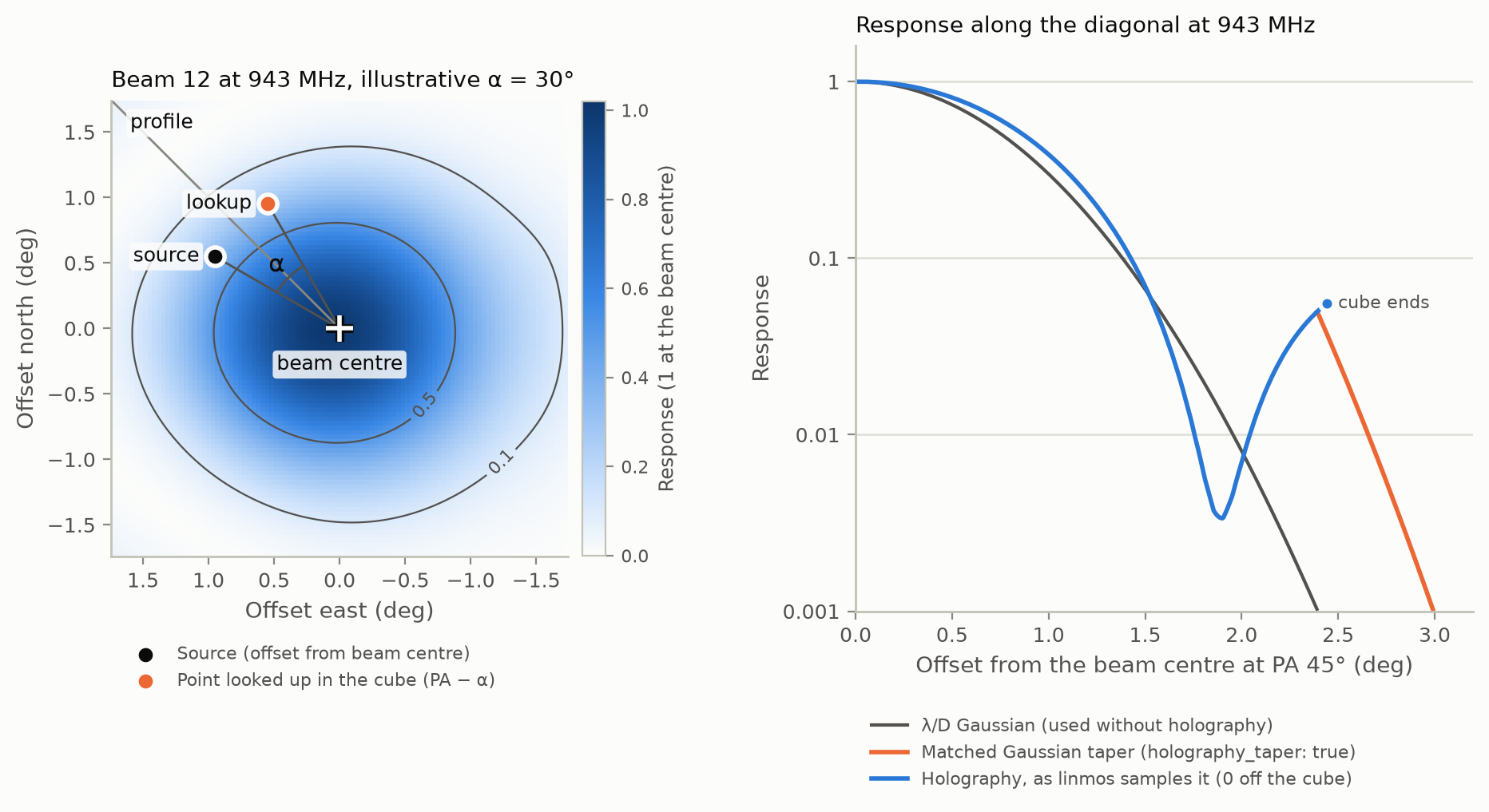
Beam 12 of the low-band holography cube SB55219 at 943 MHz. Left: the beam in
its offset grid, with east to the left. With an illustrative α of 30°, a
source at PA 60° is looked up at PA 30°. Contours are at 0.5 and 0.1. Right:
the response along the diagonal at PA 45°, out through the cube’s corner. The
measured beam is used all the way to the corner, including the sidelobe beyond
2°. With holography_taper on, a matched Gaussian takes over where the cube
ends. The plain λ/D Gaussian, used when there is no holography, is narrower
than the measured beam.
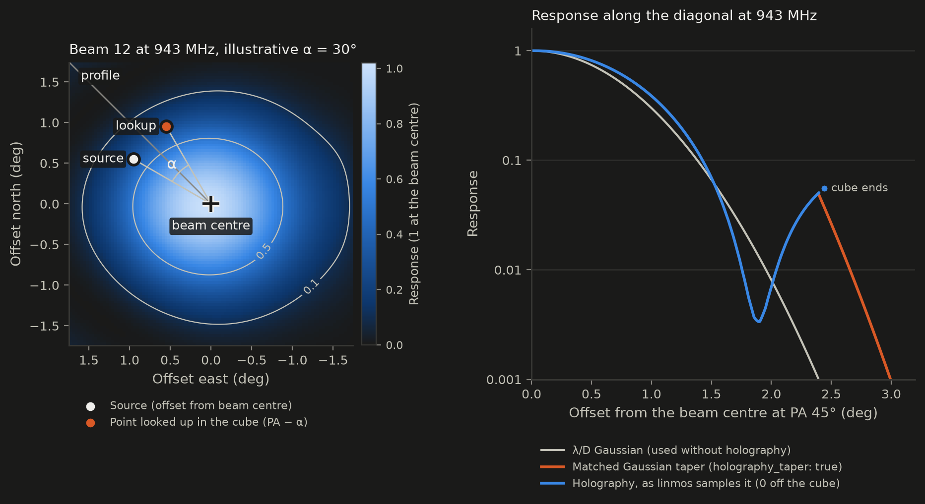
Beam 12 of the low-band holography cube SB55219 at 943 MHz. Left: the beam in
its offset grid, with east to the left. With an illustrative α of 30°, a
source at PA 60° is looked up at PA 30°. Contours are at 0.5 and 0.1. Right:
the response along the diagonal at PA 45°, out through the cube’s corner. The
measured beam is used all the way to the corner, including the sidelobe beyond
2°. With holography_taper on, a matched Gaussian takes over where the cube
ends. The plain λ/D Gaussian, used when there is no holography, is narrower
than the measured beam.
Frequency. Planes with no response at the beam centre are dropped. These are usually flagged holography channels stored as NaN; in the mid-band cube SB66096, for example, everything below 1296 MHz is NaN. The remaining planes are put in increasing frequency and interpolated linearly onto the measurement set’s channels. linmos uses the nearest plane instead, which makes no practical difference with 1 MHz planes. Channels more than half a plane beyond the usable planes take the nearest plane’s beam, and a warning says how many.
Normalisation
Each frequency plane is divided by its value at the beam centre, so the response is exactly 1 there. That matches the flux scale of the data: the bandpass is calibrated on PKS B1934−638 placed at each beam’s centre.
The cubes are not quite normalised as stored. They read about 1.005 to 1.016 at the beam centre, and peak a further 0.5–1% higher, 2–6′ away from it. linmos uses the stored values, so mosaic fluxes and this model can differ by 0.5–1.5%. A phase-only solution is not sensitive to that.
Sources beyond the edge of the cube
The cubes are small. They span about ±1.7° in the low and mid bands and ±0.9° in the high band. By default a source off the cube gets a response of 0 and is dropped, which is what linmos assumes.
With holography_taper: true, those sources are kept. Inside the cube the
measured beam is still used everywhere, exactly as linmos uses it. That
includes the corners, which reach about 1.4 times further out than the edges
and can hold real sidelobes: a few percent at 2.1–2.3° on the diagonals of the
low-band cube. For a source off the cube, follow the line from the beam
centre through the source to where it leaves the cube, one pixel inside the
edge. The response is then:
the measured value at that exit point, clipped at 0;
multiplied by how much a λ/D Gaussian falls off between the exit point and the source.
The response is therefore continuous at the edge and falls off smoothly in the source’s own direction. It is 0 where the measured value at the exit point is 0 or below. The exit point is used rather than the nearest pixel because the beam is not circular: the nearest pixel can lie in a different direction, and so a different part of the pattern. Only a Gaussian is used for the fall-off. Airy and sinc² patterns have nulls inside the cube edge in some bands, so they cannot be matched to the measured value safely.
To bring in more distant bright sources, also raise fwhm_scale_cutoff, which
sets how far out sources are looked for.
When something goes wrong
Each case below either stops with an error or logs a warning:
The MS name has no beam number. The beam is read from the MS’s
FEED1column instead, with a warning startingBEAM NUMBER NOT IN NAME. IfFEED1holds more than one beam, it stops with an error.The beam has no usable response. That is, every plane is NaN or zero at the beam centre. A warning names the cube and the beam, and that measurement set falls back to the Gaussian beam. For example, beam 12 of the high-band cube SB34422 is entirely zero. The rest of the flow carries on as normal.
The cube’s beam centre is at its edge. If the reference pixel (
CRPIX) is within a pixel of the cube’s edge, it stops with an error. ASKAP holography cubes are centred on the beam, so this means the cube is not the kind expected.Channels fall outside the usable planes. A warning gives the number of channels and the usable range; those channels take the nearest plane’s beam.
No sources are left to model. If none survive the flux and radial cuts, the flow stops with a
NoFieldSourceError. Loweringflux_cutoff, raisingfwhm_scale_cutoffor turning onholography_tapermay help.
Gaussian components and position angles
What is written for each source
Each component goes into the model file as one line, with its position, the fitted apparent spectrum and its shape:
POINT if both axes are under 1″, or if it has no position angle.
GAUSSIAN otherwise, with the major axis and minor axis in arcseconds and the orientation in degrees.
A missing position angle needs care. In NVSS, the position angle is blank
exactly when both axes are only upper limits, which is 84% of the catalogue.
Those sources are unresolved, so they are written as points. A nan
orientation would be worse than useless: addmodel would predict NaN for
every visibility, not just that source’s.
The sizes must be intrinsic (deconvolved), because the instrument’s
resolution comes from the visibilities themselves. NVSS and SUMSS list
deconvolved sizes. For a catalogue of your own, say which kind you have with
catalogue_sizes_deconvolved. If the sizes are as observed, name the per-source
PSF columns (catalogue_psf_maj_col, catalogue_psf_min_col,
catalogue_psf_pa_col) so they can be deconvolved.
The rotation α does not move sources
α only changes where in the cube a source’s beam response is read. It turns the beam pattern, not the sky. The sources’ shapes stay as the catalogue gives them, for three reasons:
addmodelpredicts with the measurement set’s own (u, v, w), which are fixed by the baselines and do not depend on how the phased array feed is turned.ASKAP’s third axis holds the feed at a fixed angle on the sky for the whole observation, so the beam does not turn during a track either. flint checks that the angle is constant.
fixmschanges the polarisation basis, not the Stokes I geometry.
North at the source versus north at the phase centre
There is one real frame difference, and it has nothing to do with α.
Catalogue position angles are measured east of north at the source.
addmodel builds each Gaussian directly in the (u, v) plane of the phase
centre, so it measures the angle from north at the phase centre. Away from
the phase centre, meridians converge, and the two norths differ by an angle η:
η = atan2(−sin δ · sin Δα, cos δ · cos δ₀ + sin δ · sin δ₀ · cos Δα)
Here δ is the source’s declination, δ₀ the phase centre’s, and Δα the difference in right ascension (source minus phase centre). η is measured east from north at the phase centre to north at the source. It is zero for sources due north or south of the phase centre. It is negative east of a northern field and positive east of a southern one, and grows roughly as Δα · sin δ.
Phase centre Dec |
1° east |
1.7° east |
1.7° at PA 45° |
|---|---|---|---|
+18.3° |
−0.33° |
−0.56° |
−0.42° |
0° |
0.00° |
0.00° |
−0.03° |
−30° |
+0.58° |
+0.98° |
+0.66° |
−60° |
+1.73° |
+2.94° |
+1.98° |
−80° |
+5.65° |
+9.55° |
+6.05° |

A source 1.7° east of a phase centre at Dec −80°, with east to the left. North
at the source (orange) is turned 9.5° from north at the phase centre (blue).
A catalogue position angle of 35° is measured from the orange arrow. Without
the correction, addmodel measures the same 35° from the blue arrow, so the
source is drawn 9.5° off. The shapes are enlarged for clarity.
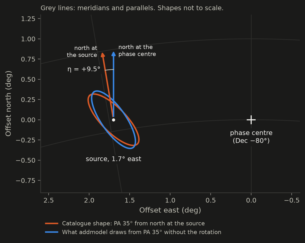
A source 1.7° east of a phase centre at Dec −80°, with east to the left. North
at the source (orange) is turned 9.5° from north at the phase centre (blue).
A catalogue position angle of 35° is measured from the orange arrow. Without
the correction, addmodel measures the same 35° from the blue arrow, so the
source is drawn 9.5° off. The shapes are enlarged for clarity.
With rotate_pa_to_phase_centre: true, η is added to each Gaussian’s
position angle as it is written, so addmodel draws the source the way the
catalogue describes it.
When to turn it on. It matters only for elongated sources in fields near the poles. Near the equator η is a fraction of a degree. A compact source looks much the same at any position angle, and phase-only calibration is barely affected by source shapes at all. It is off by default.
What it changes. Only the calibrate model file passed to addmodel. The
ds9 region file and the hyperdrive model keep the catalogue’s own position
angles, which is what those tools expect.
Configuration
The RACS-All flow reads the sky-model step’s options from the strategy file,
for self-calibration round 0: the model from the skymodel section, and the
calibration from the gaincal section. Values under defaults apply first,
and values under selfcal: 0 override them. Every option on this page:
defaults:
  skymodel:
    # Catalogue to use; unset picks SUMSS, RACS-low or NVSS by declination
    reference_name: NVSS
    # Minimum brightness, in Jy, before and after the beam is applied
    flux_cutoff: 0.02
    # How far out to look for sources, in units of λ/D at the lowest frequency
    fwhm_scale_cutoff: 1.0
    # Keep sources beyond the edge of the holography cube with a matched taper
    holography_taper: false
    # Measure position angles from north at the phase centre, as addmodel expects
    rotate_pa_to_phase_centre: false

selfcal:
  0:
    skymodel:
      holography_taper: true
    # Calibration against the sky model; always phase-only
    gaincal:
      solint: 120s
      minsnr: 3.0
      uvrange: ">200m"
      nspw: 1
The sky-model calibration is always phase-only. A calmode other than p
in its options is ignored, with a warning. Without a gaincal section,
gaincal runs on flint’s defaults: solint: 60s, minsnr: 0.0 and
uvrange: ">200m". Values under defaults: gaincal: also apply to the
regular self-calibration rounds, which each read the gaincal section of their
own round.
The flow always writes the calibrate model, and takes the catalogue directory
from --reference-catalogue-directory. To build the model from a catalogue of
your own instead, see Using your own catalogue.
Using your own catalogue
The model can be built from any catalogue astropy can read, instead of the
built-in reference catalogues. Point catalogue_path at the file in the
skymodel section of the strategy file and name its columns. Nothing is
guessed: every column and unit the model needs must be given. With
catalogue_path set, reference_name is ignored and the model does not use
the reference catalogue directory. --reference-catalogue-directory is still
required and checked, because the flow’s validation plots use it.
Each beam still gets its own model. From the one file, only sources within
fwhm_scale_cutoff × λ/D of that beam’s phase centre and brighter than
flux_cutoff are kept.
The options
Option |
Needed |
What it gives |
|---|---|---|
|
always |
The file. Its format comes from the extension ( |
|
always |
Position columns |
|
if not degrees |
Unit of the position columns |
|
always |
Flux of each component at the reference frequency |
|
if not Jy |
Unit of the flux column |
|
one of them |
The reference frequency in Hz for every source, or a column holding one per source (with |
|
no |
Component names, used only as labels. Without it, components are named |
|
no, but all three or none |
Shape: major and minor axis (FWHM) and position angle, east of north in degrees. Without them, every component is a point. |
|
if not arcsec |
Unit of the axis columns, including the PSF columns below |
|
when shapes are given |
|
|
when |
Each component’s restoring beam, used to deconvolve the observed axes |
|
no |
Spectral index and curvature. Without them, |
Things to check in your catalogue
Units are labels, not conversions. Each
*_unitoption is stamped onto its column, replacing whatever unit the file declares. If a FITS column holds mJy andcatalogue_flux_unitis left asJy, every flux is 1000 times too bright. Set each unit to what the file actually holds.Use the per-component flux (integrated flux of each Gaussian), not a peak flux or a whole-source total.
One unit for all the shape columns.
catalogue_shape_unitcovers the axis columns and the PSF columns together, so they must share a unit. If they don’t, use deconvolved axes instead.Blank shapes are fine. A component with no position angle, or with both axes under 1″, is written as a point. That matches how PyBDSF and NVSS mark unresolved sources.
Every row is used. There is no option to filter rows, so remove anything you don’t want modelled (flagged, spurious or duplicated components) before pointing the flow at the file.
Large catalogues are read in full for every beam and band. That is 108 reads for a 36-beam, three-band run. Write a copy that keeps only the columns the model uses, and if you can, only the sky around your fields:
from astropy.table import Table

columns = ["RA", "DEC", "Total_flux", "DC_Maj", "DC_Min", "DC_PA", "Gaussian_ID"]
table = Table.read("survey_components.fits")
table[columns].write("survey_components_skymodel.fits")
Example: a PyBDSF Gaussian list
PyBDSF writes RA and Dec in degrees, Total_flux per Gaussian in Jy, and
deconvolved sizes (DC_Maj, DC_Min, DC_PA) in degrees, with both axes set
to 0 for unresolved Gaussians. The reference frequency is the FREQ0 keyword
in the table header. Use the sky-plane columns, not the _img_plane ones. For
a RACS-low3 Gaussian list at 943.491 MHz:
defaults:
  skymodel:
    catalogue_path: /path/to/RACS-low3_flint_components.fits
    catalogue_ra_col: RA
    catalogue_dec_col: DEC
    catalogue_radec_unit: deg
    catalogue_flux_col: Total_flux
    catalogue_flux_unit: Jy
    catalogue_freq: 943491000.0
    catalogue_name_col: Gaussian_ID
    catalogue_maj_col: DC_Maj
    catalogue_min_col: DC_Min
    catalogue_pa_col: DC_PA
    catalogue_shape_unit: deg
    catalogue_sizes_deconvolved: true
    assumed_alpha: -0.83
    assumed_beta: 0.0
The as-observed columns (Maj, Min, PA) can’t be paired with PyBDSF’s PSF
columns here: the axes are in degrees and the PSF columns in arcseconds, and
catalogue_shape_unit has to cover both.
Building a sky model from the command line
flint_skymodel builds the same model for one measurement set. Pass
--holofile to take the beam from a holography cube; without it, the Gaussian
beam is used. It accepts every option above:
Create a calibrate compatible sky-model for a given measurement set.
usage: flint_skymodel [-h] [--holofile HOLOFILE]
                      [--reference-catalogue-directory REFERENCE_CATALOGUE_DIRECTORY]
                      [--reference-name REFERENCE_NAME]
                      [--assumed-alpha ASSUMED_ALPHA]
                      [--assumed-beta ASSUMED_BETA]
                      [--flux-cutoff FLUX_CUTOFF]
                      [--fwhm-scale-cutoff FWHM_SCALE_CUTOFF]
                      [--write-hyperdrive-model] [--write-calibrate-model]
                      [--write-ds9-region] [--holography-taper]
                      [--rotate-pa-to-phase-centre]
                      [--catalogue-path CATALOGUE_PATH]
                      [--catalogue-freq CATALOGUE_FREQ]
                      [--catalogue-freq-col CATALOGUE_FREQ_COL]
                      [--catalogue-freq-unit CATALOGUE_FREQ_UNIT]
                      [--catalogue-ra-col CATALOGUE_RA_COL]
                      [--catalogue-dec-col CATALOGUE_DEC_COL]
                      [--catalogue-flux-col CATALOGUE_FLUX_COL]
                      [--catalogue-name-col CATALOGUE_NAME_COL]
                      [--catalogue-maj-col CATALOGUE_MAJ_COL]
                      [--catalogue-min-col CATALOGUE_MIN_COL]
                      [--catalogue-pa-col CATALOGUE_PA_COL]
                      [--catalogue-sizes-deconvolved CATALOGUE_SIZES_DECONVOLVED]
                      [--catalogue-psf-maj-col CATALOGUE_PSF_MAJ_COL]
                      [--catalogue-psf-min-col CATALOGUE_PSF_MIN_COL]
                      [--catalogue-psf-pa-col CATALOGUE_PSF_PA_COL]
                      [--catalogue-alpha-col CATALOGUE_ALPHA_COL]
                      [--catalogue-beta-col CATALOGUE_BETA_COL]
                      [--catalogue-radec-unit CATALOGUE_RADEC_UNIT]
                      [--catalogue-flux-unit CATALOGUE_FLUX_UNIT]
                      [--catalogue-shape-unit CATALOGUE_SHAPE_UNIT]
                      ms
Positional Arguments
- ms
Path to the measurement set to create the sky-model for
Named Arguments
- --holofile
Holography cube to take the primary beam from. If unset, a Gaussian beam is used
Inputs for SkyModelOptions
- --reference-catalogue-directory
The reference catalogue directory that contains the known flint reference catalogues
Default:
.- --reference-name
- --assumed-alpha
Assume this to be the typical spectral index if it is not recorded in the reference catalogue
Default:
-0.83- --assumed-beta
Assume this to be the typical amount of spectral curvature should they not be in the reference catalogue
Default:
0.0- --flux-cutoff
The intrinsic brightness a source needs to be for it to be included in the sky model
Default:
0.02- --fwhm-scale-cutoff
A source needs to be within this many FWHM units from the direction of interest for it to be included
Default:
1- --write-hyperdrive-model
Should the model for hyperdrive be created. The output will have .hypderdrive.yaml suffix appended to the MS path.
Default:
False- --write-calibrate-model
Should the model for calibrate be created. The output will have .calibrate.txt suffix appended to the MS path.
Default:
False- --write-ds9-region
Should a DS9 region file be created. The output will have .ds9.reg suffix appended to the MS path.
Default:
False- --holography-taper
Keep sources beyond the edge of the holography cube, continuing the beam past the edge as a Gaussian fall-off from the edge value. Off drops them, as linmos does.
Default:
False- --rotate-pa-to-phase-centre
Measure position angles in the calibrate model from north at the phase centre, as addmodel expects, instead of from north at each source
Default:
False- --catalogue-path
Path to a user-supplied catalogue file. If set, takes precedence over reference_catalogue_directory/reference_name. Column names/units below are never guessed.
- --catalogue-freq
Reference frequency, in Hz, of catalogue_path’s flux column, used for every source. Ignored if catalogue_freq_col is set. One of catalogue_freq/catalogue_freq_col is required whenever catalogue_path is set.
- --catalogue-freq-col
Per-source reference-frequency column in catalogue_path. If set, overrides catalogue_freq with a per-row value instead of one value for the whole catalogue.
- --catalogue-freq-unit
Astropy unit string for catalogue_freq_col
Default:
'Hz'- --catalogue-ra-col
RA column in catalogue_path. Required whenever catalogue_path is set – never guessed
- --catalogue-dec-col
Dec column in catalogue_path. Required whenever catalogue_path is set
- --catalogue-flux-col
Flux column in catalogue_path. Required whenever catalogue_path is set
- --catalogue-name-col
Source name column in catalogue_path. If unset, names are synthesised (src0, src1, …)
- --catalogue-maj-col
Major-axis column in catalogue_path. None disables shape info (point sources). Must be set together with catalogue_min_col/catalogue_pa_col
- --catalogue-min-col
Minor-axis column in catalogue_path, paired with catalogue_maj_col
- --catalogue-pa-col
Position-angle column in catalogue_path, paired with catalogue_maj_col. Always degrees
- --catalogue-sizes-deconvolved
Whether catalogue_maj_col/catalogue_min_col are already intrinsic (PSF-deconvolved) sizes, ready to use directly in the sky model, or as-observed (PSF-convolved) sizes that must be deconvolved first. Required whenever catalogue_maj_col is set – never guessed
- --catalogue-psf-maj-col
Per-source PSF major-axis column in catalogue_path, used to deconvolve catalogue_maj_col/catalogue_min_col when catalogue_sizes_deconvolved is False. Required in that case – there is no pipeline restoring beam to fall back on here
- --catalogue-psf-min-col
Per-source PSF minor-axis column, paired with catalogue_psf_maj_col
- --catalogue-psf-pa-col
Per-source PSF position-angle column, paired with catalogue_psf_maj_col. Always degrees
- --catalogue-alpha-col
Spectral index column in catalogue_path. If unset, falls back to assumed_alpha
- --catalogue-beta-col
Spectral curvature column in catalogue_path. If unset, falls back to assumed_beta
- --catalogue-radec-unit
Astropy unit string for catalogue_ra_col/catalogue_dec_col. Always applied explicitly, never inferred from the file
Default:
'deg'- --catalogue-flux-unit
Astropy unit string for catalogue_flux_col
Default:
'Jy'- --catalogue-shape-unit
Astropy unit string for catalogue_maj_col/catalogue_min_col/catalogue_psf_maj_col/catalogue_psf_min_col
Default:
'arcsec'